Author: Yiming Ma, Yao Zeng, and Anthony Lee Zhang, Source: The University of Chicago, Translated by: Qian Jiayan
1. Introduction
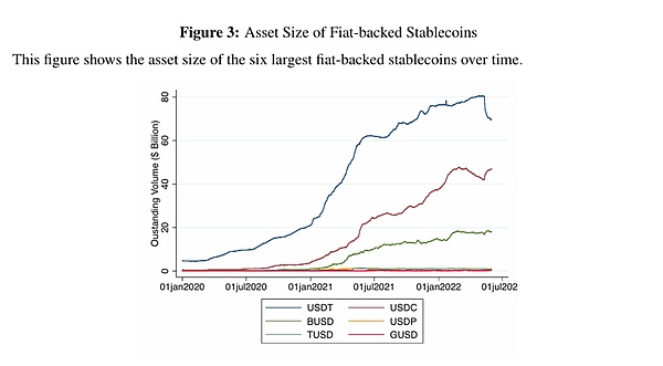
Fiat-backed stablecoins are blockchain assets whose value is claimed to be stable at $1. This price stability is achieved by promising to back each stablecoin token with at least $1 in USD-denominated assets, such as bank deposits, Treasury bills, corporate bonds, and loans. The market capitalization of the six largest USD-backed stablecoins has grown from $5.6 billion at the beginning of 2020 to over $130 billion at the beginning of 2022. The potential for stablecoins to become a widely accepted means of payment, competing with fiat currencies and bank deposits, has sparked active discussions on how to mitigate potential risks to financial stability and what the optimal regulatory framework should be.
An ideal stablecoin would always trade at a stable $1 and would not experience panic runs. However, stablecoins hold illiquid assets but promise a fixed redemption value of $1. Unlike money market funds (MMFs) or commercial banks, this $1 redemption is limited to specific institutional arbitrageurs. The vast majority of investors can only trade stablecoins on secondary market exchanges, similar to investors trading ETF shares in the secondary market. These investors trade at the secondary market price, which often fluctuates around $1 due to supply and demand pressures in the market. Since stablecoin prices are determined in equilibrium, when and why would stablecoin investors want to run? How do stablecoin price deviations relate to their run risk?
This paper answers these questions by constructing a framework for the structure of stablecoin markets, showing how issuers, arbitrageurs, and customers interact to determine the stability of stablecoin prices and the likelihood of panic runs. Our findings provide important insights into the optimal regulation of stablecoins. These insights are particularly relevant because different jurisdictions have recently proposed different regulatory proposals for stablecoins, and these proposals are not always consistent with each other.
First, some proposals require stablecoin issuers to offer unlimited direct redemptions to all investors, which would effectively eliminate the current two-tier market structure. Such policies would indeed promote price stability through more competitive arbitrage. However, in cases where stablecoins are allowed to continue to transform liquidity, our model suggests that more efficient arbitrage would also amplify the risk of panic runs. In contrast, imposing redemption fees on arbitrageurs would reduce run risk by limiting arbitrage, but at the expense of price stability.
Second, many policy proposals impose constraints on the safety and liquidity of stablecoin issuers’ reserve assets. Our results suggest that reserve asset policies should be coordinated with policies governing redemptions, as these factors jointly determine both price stability and run risk outcomes.
Third, allowing dividend payments further improves the price stability of stablecoins and may reduce the risk of runs. In summary, while price stability and low run risk are both desirable features of stablecoins, they are inherently different and respond differently to policy interventions.
2. Stablecoin Details
Stablecoins are blockchain assets whose value is claimed to be stable at $1. Blockchain assets can be self-custodial: users can directly hold, send and receive stablecoins using crypto wallet software such as MetaMask. These stablecoins are not stored in any trusted intermediaries: instead, a "private key" (a long numeric code that is usually only saved on the user's hardware device) is used to prove to the blockchain network that the user owns their stablecoins and instruct the network to take actions such as transferring stablecoins to other wallets. Others cannot access an individual's private key, so they cannot take funds from an individual's wallet.
Compared to other blockchain assets such as Bitcoin, the notable feature of stablecoins is relative price stability. The largest stablecoin issuers attempt to achieve price stability by promising to back each stablecoin token with at least $1 of off-chain USD assets. These fiat-backed stablecoins have experienced rapid expansion over the past few years. In two years, the total assets of the six largest fiat-biased stablecoins have grown from $5.6 billion at the beginning of 2020 to over $130 billion at the beginning of 2022 (Figure 3). The two largest stablecoins are Tether (USDT) and Circle USD Coin (USDC), and in January 2022, their combined market capitalization reached $76.4 billion, accounting for more than 50% of the total market size. Binance USD (BUSD), Paxos (PUSD), TrueUSD (TUSD), and Gemini USD (GUSD) are much smaller.
In the rest of this section, we provide an overview of the uses of stablecoins and the stablecoin market structure.
2.1 Purpose of Stablecoins
Stablecoins are a fairly low-cost way to transact and hold USD assets. If a remitter in country A sends money to a recipient in country B, she can buy stablecoins with country A’s fiat currency on a cryptocurrency exchange, withdraw those stablecoins to her own cryptocurrency wallet, and then send them to the recipient’s wallet in country B. The recipient can then deposit those funds on a cryptocurrency exchange in her home country, convert the stablecoins to fiat currency, and then withdraw the fiat currency. Sending stablecoins from one cryptocurrency wallet to another is relatively quick and inexpensive. As of January 2023, transactions to send stablecoins on the Ethereum blockchain complete in under a minute and cost about $1 per transaction, regardless of the amount of stablecoins being sent. Stablecoins can also be used as a store of value; they can be held in a crypto wallet for free and indefinitely.
Thus, while stablecoins cost more to use than well-functioning banking services in developed countries, they are competitive in contexts where traditional financial infrastructure does not function well. For example, stablecoins are gaining widespread adoption in environments where transactions must cross borders, where capital controls and financial repression are prevalent, where inflation is high, or where trust in financial intermediaries is low.
Stablecoins are also used to trade with other blockchain smart contracts. For example, market participants can use stablecoin tokens to purchase other blockchain tokens such as ETH, MKR, or UNI through automated market maker protocols such as Uniswap. Market participants can also lend stablecoin tokens on lending protocols such as Aave and Maker to earn positive interest rates, or use these assets as collateral to borrow other assets. In a sense, stablecoins provide a secure means of storing value and a medium of exchange for the blockchain ecosystem.
2.2 Market Structure
Stablecoin tokens are created ("minted") or redeemed ("destroyed") in the primary market in the form of U.S. dollar cash, as shown on the left side of Figure 4. To create a stablecoin token, an arbitrageur sends $1 to the issuer, who then sends one stablecoin token to the crypto wallet of a market participant. Similarly, to redeem a stablecoin token, the issuer sends $1 to the market participant's bank account, for every stablecoin token sent by the market participant to the issuer's crypto wallet, such as through a bank transfer. The primary market for stablecoins is similar to money market funds in the traditional financial system.
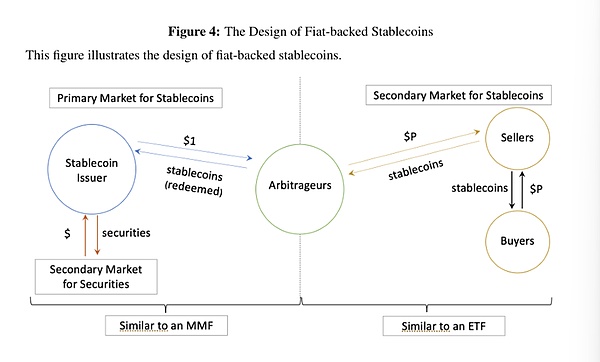
Most market participants cannot become arbitrageurs to redeem and create stablecoin tokens, and stablecoin issuers differ in the ease and cost of primary market entry for market participants. According to market participants, USDC allows general businesses to register as arbitrageurs, while USDT requires a lengthy due diligence process and places restrictions on where arbitrageurs can register. In addition, USDT has a minimum transaction size of $100,000 and charges the greater of 0.1% and $1,000 for each redemption.
Most market participants exchange existing stablecoins for fiat currencies on the secondary market. Cryptocurrency exchanges allow investors to deposit USD and then trade USD for stablecoins with other market participants. Therefore, the price of stablecoin tokens on the secondary market is determined by supply and demand. When stablecoin selling surges, the secondary market price falls, but it does not directly lead to the liquidation of reserve assets. In this way, the buying and selling of stablecoins on the secondary market is similar to the trading of ETF shares on competing exchanges.
However, selling pressure in the secondary market may spread to the primary market through arbitrageurs. When the secondary market price falls below $1, arbitrageurs can profit by purchasing stablecoin tokens in the secondary market and exchanging them for $1 at a 1:1 ratio with the stablecoin issuer in the primary market. Through this arbitrage, the $1 redemption value of the primary market stablecoin will pull the trading price of the secondary market stablecoin towards $1. At the same time, this arbitrage process also means that when the stablecoin issuer liquidates the reserves to meet the cash redemptions of arbitrageurs, the selling pressure of secondary market investors will eventually trigger the sale of reserve assets. If illiquid reserve assets are sold at a discount, the cost of these fire sales may be particularly high.
3. Data
In this section, we explain our main data sources.
Primary market data:
The core dataset used in this analysis is data on every stablecoin creation and redemption event for the six largest fiat-backed stablecoins (USDT, USDC, USDP, TUSD, and GUSD) on the Ethereum, Avalanche, and TRON blockchains. We obtain this data from each blockchain’s “chain explorer” websites, which process transaction-level blockchain data into a usable format. We use Etherscan for Ethereum data, Snowtrace for Avalanche data, and Tronscan for TRON data. The data extraction process allows us to see the precise timestamp of each stablecoin creation and redemption event, the number of stablecoins redeemed or created, and the wallet addresses of the entities involved in the stablecoin creation and redemption. The blockchain only records wallet addresses, and the same institution may have multiple wallet addresses. During the data collection process, we merge wallets whose Etherscan tags clearly indicate that they belong to the same institution. However, this process may not be exhaustive, so the arbitrage concentration calculated in this article should be regarded as a lower bound on the true arbitrage concentration.
Secondary market data:
For each stablecoin, we extract hourly closing prices of direct USD-stablecoin transactions from several major exchanges, including Binance, Bitfinex, Bitstamp, Bittrex, Gemini, Kraken, Coinbase, Alterdice, Bequant, and Cexio. The differences in stablecoin prices between major exchanges are generally negligible, so the price series is not materially affected by the weights we assign to different exchanges. We winsorize secondary market prices at the 1% level.
4. Other facts about stablecoins
In this section, we present a new set of facts about stablecoins to inform our model and calibration.
4.1 Secondary Market Price
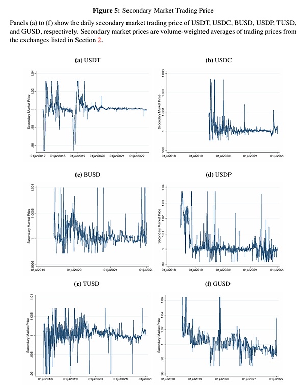
Fact 1: Stablecoins typically trade at a price that deviates from $1 in the secondary market.
Figure 5 shows the trading prices of different stablecoins on the secondary market over time. We observe that secondary market prices are rarely fixed at $1. Instead, across our sample of stablecoins, stablecoins trade at a discount 27.2% to 41.6% of the time and at a premium 57.3% to 72.8% of the time (see Table 1a). The magnitude of these price deviations varies across stablecoins. While USDT has an average discount of 54 basis points, USDC has an average discount of just 1 basis point. BUSD, TUSD, and USDP also have lower average discounts than USDT, while GUSD has the highest average discount. The magnitude of the median discount is generally smaller than the average discount, but the cross-sectional differences remain similar. For example, the median discount for USDT is 11 basis points, while the median discount for USDC is less than 1 basis point. The magnitude is also reduced when considering a common sample period.
Starting in January 2020, when all six stablecoins were traded, the differences between the currencies still exist, with USDT trading at a larger average discount than USDC (see Table 1b). The average and median premiums also show significant differences in the cross-section.
4.2 Primary Market Concentration
Fact 2: Redemption and creation of stablecoins in the primary market are performed by a small group of arbitrageurs, the concentration of which varies from stablecoin to stablecoin.
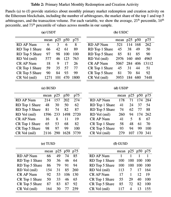
Table 2 shows the characteristics of monthly primary market redemption and creation activity for different stablecoins on the Ethereum blockchain. On average, USDT has only 6 arbitrageurs participating in redemptions per month, while USDC has 521. The market share concentration of arbitrageurs is generally higher, but still varies by stablecoin. The largest arbitrageur of USDT completes 66% of all redemption activities, while the largest arbitrageur of USDC completes 45%. In contrast, most other stablecoins fall between USDT and USDC in terms of the number of arbitrageurs and arbitrageur concentration. In terms of trading volume, the average monthly redemption volume of USDT is $577 million, while that of USDC is $2.976 billion. In contrast, the total outstanding tokens of USDT are 1.5 to 2 times that of USDC. Therefore, the larger number of arbitrageurs and lower concentration of USDC are also associated with higher redemption volumes relative to total asset size. The creation volume is larger and there are relatively more arbitrageurs participating in creation, but the trends and arbitrage concentrations remain similar across different stablecoins.
4.3 Secondary Market Prices and Primary Market Concentration
Fact 3: Stablecoins with a more concentrated group of arbitrageurs will experience more obvious price deviations in the secondary market.
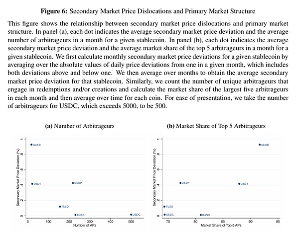
Next, we analyze the relationship between price deviation and arbitrageur concentration. For a given stablecoin, we calculate the monthly secondary market price deviation by averaging the absolute value of the daily price deviation from 1 in a given month, including deviations above and below 1. We then average the data across months to get the average price deviation for that stablecoin. Similarly, we count the number of unique arbitrageurs who participated in redemption and/or minting, and calculate the market share of the top five arbitrageurs in each month and the average over time for each stablecoin.
The results are shown in Figure 6a. A clear negative trend emerges: stablecoins with fewer arbitrageurs (such as USDT) have higher average deviations from 1 in secondary market prices compared to stablecoins with more arbitrageurs (such as USDC). Another way to measure arbitrageur concentration is through the market share of the largest arbitrageurs. In Figure 6b, we repeat the analysis using the market share of the top five arbitrageurs. The relationship is positive. Stablecoins where the top five arbitrageurs consistently account for a larger share of total redemptions and minting have higher average price deviations than other stablecoins with lower arbitrageur concentration. In other words, it seems that higher arbitrage competition is associated with less secondary market price misalignment.
4.4 Liquidity Conversion
Fact 4: Stablecoins achieve varying degrees of liquidity conversion by investing in illiquid assets.
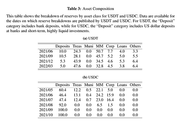
Stablecoin issuers hold USD-denominated assets with varying degrees of illiquidity as reserves. Table 3 shows the composition of USDT and USDC reserve assets on the reporting date. In general, the reserve assets of USDT and USDC are not completely liquid, with USDT's reserve assets being more illiquid.
V. Theoretical Framework
5.1 Stablecoin runs and centralization of arbitrage
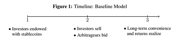
The baseline economic model is based on the work of Diamond and Dibvig (1983) and has three time points, t = 1, 2, 3, and no time discounting. This article provides a timeline in Figure 1 to illustrate the economic model:
There are two groups of risk-neutral participants :
1) A competing group of stablecoin investors indexed by i, and
2) A group of n stablecoin arbitrageurs.
There are two types of assets :
1) US dollar, which is risk-free, highly liquid and used as a unit of account;
2) An illiquid and potentially productive reserve asset.
Investors collectively hold stablecoins that are initially backed by reserve assets at t = 1. The initial value of the reserve assets is normalized to $1. At t = 2 and t = 3, investors decide whether to liquidate their stablecoins early at t = 2 (which could trigger a run) or hold them until maturity at t = 3 to earn a long-term yield (as we discuss below). Unlike bank depositors, stablecoin investors cannot redeem their stablecoins directly from the issuer. Instead, they sell their stablecoins to arbitrageurs in the secondary market at t = 2, following the mechanisms proposed by Jacklin (1987) and Farry, Golosov, and Tsywinsky (2009), who then redeem them for cash from the issuer. As in these models, investors sell stablecoins by submitting market orders independently. This assumption is consistent with empirical evidence that retail investors are more likely to use market orders, especially when spreads are narrow (Kelly and Tetlock, 2013), as is the case with stablecoins. In this paper, λ is used to represent the proportion of investors who sell stablecoins at the market price p2.
Arbitrageurs bid competitively in a double auction to determine the price p2 at which investors sell λ stablecoins, taking into account the amount they expect to be able to redeem from the issuer. In the baseline model, it is assumed that arbitrageurs cannot hold net inventories, so their net redemptions in the primary market at t = 2 must equal their purchases in the secondary market. In Appendix C.1, we show that this assumption is consistent with the empirical observation that the vast majority of arbitrageurs hold very small amounts of stablecoins. Arbitrageurs face quadratic inventory costs: arbitrageur j incurs the cost of arbitrage zj units of stablecoins from the secondary market to the primary market, where χ can be viewed as a measure of the arbitrageur's balance sheet capacity: when χ is high, the inventory cost is low.
When deciding whether to liquidate their stablecoins early, investors at t = 2 receive private information about economic fundamentals at t = 3. Following the global game literature, each investor i receives a private signal θi = θ + εi at t = 2, where the noise term εi is independent and uniformly distributed on [−ε,ε]. This paper focuses on arbitrarily small noise, i.e., ε→ 0, but the model results also hold outside the limit.
Fundamentals θ reflect the overall risk level and determine the long-term value of the stablecoin at t = 3. With probability 1 - π(θ), the economy enters a bad state: the reserve asset fails, and investors receive neither any nominal return nor any long-term benefit from holding a stablecoin backed by worthless assets. With probability π(θ), the economy enters a good state: the reserve asset generates a positive value of R(ϕ) ≥ $1, which belongs to the issuer. The stablecoin continues to operate, and the remaining 1 - λ investors receive a long-term benefit η > 0 per stablecoin, and an initial value of 1 per unit of remaining reserve assets. This long-term benefit η can be explained by the return on investors lending stablecoins.
Following backward induction, we first consider p2, the price that investors receive when they liquidate their stablecoins early. In the main paper, we derive the inverse demand function generated by competitive bidding by arbitrageurs. If arbitrageurs bid strategically, our model is similar to the setting of Klemperer and Meyer (1989), which has multiple equilibria. However, under the equilibrium selection rule that selects the equilibrium bid curve that is closest to the standard linear solution, our core economic insight about how arbitrage power affects stablecoin prices remains unchanged.
This paper derives the inverse demand function by setting price equal to marginal cost.
Assuming λ ≤ 1−ϕ, which means the issuer is solvent, an arbitrageur who buys zj units at price p2 in the secondary market and redeems them in the primary market will receive:
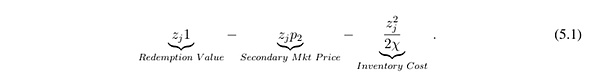
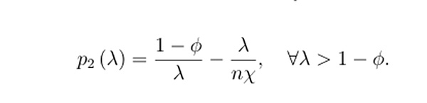
In any symmetric equilibrium, the total stock absorbed by each arbitrageur is z∗ j = λ n. If the issuer treats the price as given, in order for z∗ j to be the optimal amount to absorb, the price must be equal to the marginal value of absorbing an additional amount of stablecoins at z∗ j. That is, taking the derivative of (5.1) with respect to zj, setting it equal to 0, and then solving for p2 yields:
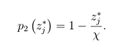
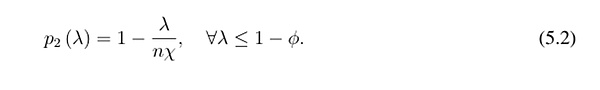
In words, the price is the marginal redemption value 1 minus the marginal inventory cost z∗ j χ. Substituting z∗ j = λ n in the symmetric equilibrium yields
In the case of insolvency, λ > 1 - ϕ, each unit of the stablecoin can only be redeemed at its liquidation value (1 - ϕ)/λ. Since investors submit market orders, the redemption value does not depend on the quantity chosen by the arbitrageur. Therefore, the arbitrageur's profit is corrected to
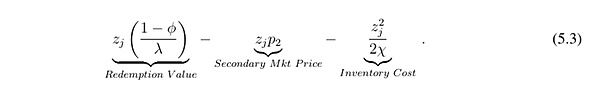
Likewise, in a symmetric equilibrium, the price must equal the marginal value of the extra quantity absorbed by the arbitrageur. Taking the derivative of (5.3) with respect to zj, setting it equal to 0, and substituting zj∗ = λn, we obtain
The only difference from (5.2) is that the redemption value is modified to (1−ϕ)/λ. We summarize these results in the following lemma.
Lemma 1. The secondary market price of a stablecoin at t = 2 is given by:
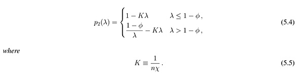
Lemma 1 shows that for any total redemption amount λ > 0, p2 decreases with increasing K and increases with increasing χ and n. Intuitively, when arbitrageurs are better capitalized (higher χ) and more numerous (higher n), secondary market prices are less affected by investor sell-offs. We call K the arbitrage capacity, and it plays a central role in the analysis because it measures the slope of secondary market demand when the issuer remains solvent. Arbitrageurs' bids create a downward-sloping demand curve for stablecoins, and the slope becomes steeper when n or χ increases, reducing the price impact of stablecoin sell-offs.
Note also that p2 is strictly decreasing with λ everywhere: the more investors sell, the lower the price. This is important because it generates strategic substitutability in investors’ selling decisions: an investor may expect to receive less from selling when many other investors are selling, thus dissuading him from selling. This force contrasts with strategic complementarity in classic bank run models (e.g., Diamond and Dybvig, 1983), where depositors receive a fixed amount of the value of their deposits when they withdraw.
Next, this paper studies the situation when t=3.
The global game framework can solve the unique equilibrium for any basic parameter value. In theory, we can get:
Proposition 1: There exists a unique threshold equilibrium in which investors sell stablecoins if the signal they receive is below the threshold θ∗, and do not sell otherwise.
Proposition 1 shows that there exists a unique threshold equilibrium for the model with private and noisy signals for investors. An investor’s liquidation decision is uniquely determined by its signal: it sells the stablecoin at t = 2 if and only if its signal is below a certain threshold. In other words, when the signal is at the threshold, there is indifference between selling and holding. Given that there is a unique run threshold, we can show that the indifference condition implies the following Laplace equation:

Solving the Laplace equation yields an analytical solution to the operating threshold and provides an intuitive comparative static analysis of the risk of stablecoin runs:
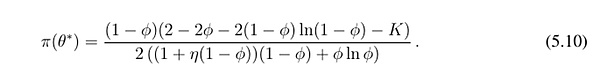
Proposition 2: The operating threshold is given by:
i). The operation threshold, that is, the operation risk, decreases with the increase of K (that is, it increases with the increase of n and increases with the increase of χ).
ii). The run threshold, i.e., the run risk, increases if and only if

where g(ϕ) is continuous and strictly decreasing in ϕ and satisfies limϕ→0 g(ϕ) > 0.
A core theoretical result is the first part of Proposition 2, which shows that more efficient arbitrage, i.e., smaller values of K, exacerbates run risk.
The second part of Proposition 2 shows that when g(ϕ) > K, the higher the level of stablecoin liquidity conversion, the higher the run risk. For a given K, this condition holds when ϕ is sufficiently small. Intuitively, when stablecoins hold more illiquid reserve assets, the first-mover advantage among investors increases, because investors who choose not to sell will have to involuntarily bear the higher liquidation costs triggered by selling investors.
5.2 Price stability and optimal stablecoin design
After analyzing the operational risks of stablecoins and their relationship to arbitrage concentration, we extend the baseline model by incorporating the price stability of stablecoins at t = 1 and the optimal design choices of issuers in the pre-trade game at t = 0.
The specific reasoning process is detailed in the original text. Regarding the optimal choice of stablecoin issuers for the concentration of arbitrageurs, the following results are obtained:
Proposition 3: Assuming G is linear and ϕ is small enough so that (5.11) holds, then the issuer's optimal choice of K decreases with ϕ: if the liquidity of the reserve assets is less, then the issuer will optimally choose a more concentrated arbitrage department.
Proposition 3 stems from the trade-off between price stability and financial stability. Stablecoin issuers choose arbitrage concentration K to balance the benefits of reducing run risk with the costs of reducing price stability. When asset illiquidity φ is high, run risk increases. At this point, issuers should be more willing to sacrifice price stability to limit run risk, resulting in a higher optimal value of K.
VI. Policy Impact
Several jurisdictions have paid more attention to the optimal regulation of stablecoins. Regulators and market participants want stablecoins to have both low run risk and price stability. Our framework emphasizes that these two desirable goals are distinct from each other and driven by different economic forces. In particular, we highlight the trade-off between price stability and financial stability and show that some policies may achieve one goal at the expense of the other. In this section, we apply model predictions to illustrate what the proposed regulation of stablecoin redemption, reserves, and interest payments would imply for price stability and financial stability.
After a series of analyses, this paper finds that dividend issuance may have other effects. For example, dividend issuance may intensify price competition among stablecoin issuers, which may encourage new entrants and improve allocation efficiency. Stablecoins that issue dividends may also be classified as securities under U.S. securities laws and face regulatory risks. We leave the analysis of these and other factors to future research.
VII. Conclusion
This article analyzes the trade-off between stablecoin run risk and price stability. From a macro perspective, stablecoin runs stem from liquidity conversion. Stablecoin issuers hold illiquid assets while offering arbitrageurs the option to redeem stablecoins at a fixed price of $1 in the primary market. This liquidity mismatch spreads from the primary market and can trigger the possibility of runs by secondary market investors even if there are exchanges trading.
Importantly, the risk of stablecoin runs is mediated by the market structure of the arbitrageur sector, which acts as a "firewall" between the secondary and primary markets. When the arbitrageur sector is more efficient, shocks from the secondary market are transmitted to the primary market more effectively. The price stability of stablecoins is thus improved, but the first-mover advantage of sellers is also higher, increasing the risk of runs. If the arbitrageur sector is less efficient, shocks from the secondary market are less effectively transmitted. Price stability is affected, but the risk of runs is reduced, because the price impact of stablecoin transactions in the secondary market inhibits panic selling by market participants.
The findings of this paper have important policy implications. Although regulators and market participants both want stablecoins to have both low run risk and maintain price stability, these two ideal goals are different from each other and are driven by different economic forces. In particular, allowing unlimited redemptions will increase arbitrage efficiency, which will help improve price stability, but may come at the cost of higher run risk. When discussing whether stablecoins should be allowed to distribute income to investors in the form of dividends, it is also necessary to consider the inhibitory effect of dividend payments on run risk. Overall, considering both price stability and run risk when designing regulatory measures is crucial for the future smooth operation and security of the stablecoin industry.